Sampling

1. Sampling Theory

Sampling: takes discrete sample values from functions defined over continuous domains and then uses those samples to reconstruct new functions that are similar to the original. The sampling and reconstruction process involves approximation and cannot capture all of the information from the continuously defined image function, so it introduces error know as aliasing including jagged edges or flickering in animations.

1.1 Understanding Pixels

• Pixels that constitute an image are point samples of the image function at discrete points on the image plane.

• The pixels in the final image are defined at discrete integer $(x, y)$ coordinates on a pixel grid, so we need to map the continuous floating-point $(x, y)$ positions generated by $Sampler$s to the discrete integer coordinate. Rounding continuous coordinates to the nearest discrete coordinate results in $\frac 12$ offsets for a given discrete pixel range. For example, given a discrete coordinates spanning a range $[x_0, x_1]$, the set of continuous coordinates that covers that range is $[x_0 - \frac 12, x_1 + \frac 12)$.

  By truncating the continuous coordinates $c$ to discrete coordinates and then convert it back to continuous: $c = \lfloor c \rfloor + \frac 12$, the range of continuous coordinates for the discrete range $[x_0, x_1]$ is naturally $[x_0, x_1 + 1)$, to simplify the relative code.

1.2 Sampler

It is useful to generalize higher dimensional sample vectors, however, to be simple, we take 2D samples as examples. For each pixel being sampled in an image, sampler may generate multiple samples and emit a ray from each of this sample position. Get multiple radiance values by path tracing. Finally, based on Monte Carlo method, average the radiances to get the color of the checked pixel. In the following, the pixel $(8, 6)$ is being sampled, and there are two image samples in the pixel area, $(x_i, y_i)$ means the offset of the sample within the pixel.

2. Stratified Sampling

2.1 Key Idea

By subdividing the sampling domain into nonoverlapping regions and taking a single sample from each one, it is less likely to miss important features of the image entirely.

2.2 Stratified Sampler

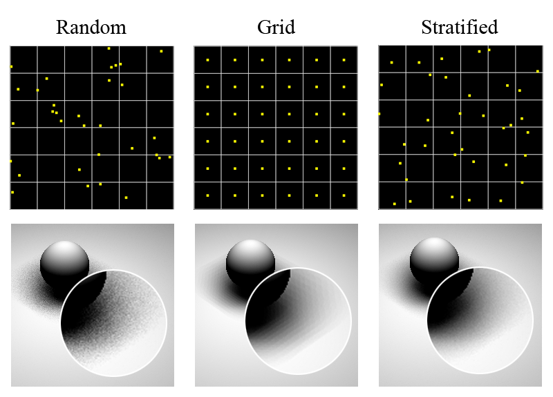
The stratified sampler places each sample at a random point inside each stratum by jittering the center point of the stratum by a random amount up to half the stratum’s width and height. This gives a better overall distribution than the purely random pattern.

2.3 Comparison of Sampling Techniques

• Random Sampling:

  It takes a random pattern which is ineffective with many clumps of samples that leave large sections of the image poorly sampled.

• Grid Sampling:

  It takes a uniform stratified pattern which is better distribution but can exacerbate aliasing artifacts.

• Stratified Sampling:

  It takes a stratified jittered pattern which can turn aliasing from the uniform pattern into high-frequency noise while still maintaining the benefits of stratification.

3. Warping 2D Samples to 3D

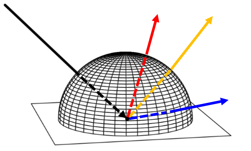
The reason why we need to warp 2D sample point $(\xi_1, \xi_2)$ to 3D point $(x, y, z)$ is that, we will need to sample points over a designated surface, like a hemisphere, when doing path tracing. For the diffuse surface, incident rays will be sampled uniformly on the unit sphere, the following inset only show 3 sample vectors as an example.

Also, when mapping 2D points onto the surfaces of various 3D shapes, it is necessary to maintain the relative spacing of the 2D points, such that the properties and benefits of the stratification will be preserved.

3.1 Uniformly Sampling a Hemisphere

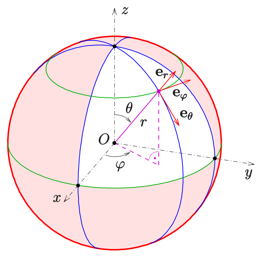
With the formula to convert the spherical coordinate to Cartesian coordinate, it is easy to do uniformly sampling a hemisphere. Given a unit sphere with the radius equal to 1,

\[\begin{cases} x &= sin\theta cos\phi \newline y &= sin\theta sin\phi \newline z &= cos\theta \end{cases}\]

Because a uniform distribution means that the density function is a constant and must integrate to one over its domain. For choosing a direction on the hemisphere uniformly with respect to solid angle, the density function $p(w) = \frac 1{2\pi}$. Given $\theta = cos^{-1} \xi_1$, $\phi = 2\pi\xi_2$, we can get the final sampling formula:

\[\begin{cases} x &= cos(2\pi\xi_2) \sqrt{1 - \xi_1^2} \newline y &= sin(2\pi\xi_2) \sqrt{1 - \xi_1^2} \newline z &= \xi_1 \end{cases}\]

3.2 Uniformly Sampling a Disc

\[\begin{cases} r = \sqrt{\xi_1} \newline \theta = 2\pi\xi_2 \end{cases} \Rightarrow \begin{cases} x = rcos\theta \newline y = rsin\theta \end{cases}\]

If set $r = \xi_1$, samples will be clumped near the center of the circle.

3.3 Cosine-Weighted Hemisphere Sampling

It is often useful to sample from a distribution that has a shape similar to that of the integrand being estimated. Considering the light transport equation (LTE):

\[L_o (p, \omega_o) = L_e(p, \omega_o) + \int_{S^2} f(p, \omega_o, \omega_i) L_i(o, \omega_i) \color {red}{ |cos\theta_i| } d \omega_i\]

Cosine-weighted Sampling: generates samples (or direction vectors) that are more likely to be close to the top of the hemisphere, where the cosine term has a larger value, than the bottom, where the cosine term is small. Therefore, each sample has a more meaningful contribution to the overall sum.

Malley’s method: generates the cosine-weighted points:

Choose points uniformly from the unit disk and then generate directions by projecting the points on the disk up to the hemisphere above it: given the coordinates $(x, y)$ of a point on the disc, get the z-coordinate of the projected point by $z = \sqrt{1 - x^2 - y^2}$.

Why does Malley’s method work?

If we pick two areas of equal size on the disc and project them to the hemisphere, the area nearer to the edge becomes much larger. Points that were close together on the disc will be spread significantly when projected to the area near the hemisphere’s edge, while points will maintain approximate spacing near the pole, which has the effect of clustering samples near the hemisphere pole.

4. Importance Sampling

Importance sampling is a variance reduction technique that exploits the fact that the Monte Carlo estimator

\[F_N = \frac 1N \sum_{i = 1}^N \frac{f(X_i)}{p(X_i)}\]

converges more quickly if the samples are taken from a distribution $p(x)$ that is similar to the function $f(x)$ in the integrand.
The basic idea is that by concentrating work where the value of the integrand is relatively high, an accurate estimate is computed more efficiently. As long as the random variables are sampled from a probability distribution that is similar in shape to the integrand, variance is reduced.

Why need the importance sampling? For example, considering the right part of the LTE equation. If a direction is randomly sampled that is nearly perpendicular to the surface normal, the cosine term will be close to 0, so all the expense of evaluating the BSDF and tracing a ray to find the incoming radiance at that sample location will be essentially wasted. In general, it is better to reduce the likelihood of choosing directions near the horizon, i.e., to choose more “important” samples (sampled from distributions that match other factors of the integrand).

References

• Matt Pharr, Wenzel Jakob, and Greg Humphreys. Physically Based Rendering: From Theory To Implementation